
Ray casting is a fascinating concept that isn’t overly complex to grasp. However, finding high-quality learning materials on the subject can be a challenge. We’ll delve into the mathematical aspects, making it easy for you to integrate into your future projects. I’ll explain things clearly, covering potential challenges and pitfalls. We’ll also explore optimization strategies, such as the significant advantages of using spatial hash maps. Keep in mind that the demos are intentionally kept simple; the goal is to understand the concept rather than delve into intricate coding details.
What is ray casting
Ray casting is the most basic of many computer graphics rendering algorithms that use the geometric algorithm of ray tracing. Ray tracing-based rendering algorithms operate in image order to render three-dimensional scenes to two-dimensional images… The idea behind ray casting is to trace rays from the eye, one per pixel, and find the closest object blocking the path of that ray – think of an image as a screen-door, with each square in the screen being a pixel. This is then the object the eye sees through that pixel. — Wikipedia on Ray casting
Let me break it down. Ray casting is a crucial and widely-used method to figure out if certain objects (polygons) are visible. This is done by tracing rays from the eye (like the player’s hero) to every pixel (though not exactly in our case - more on that later) and identifying the closest intersections with objects.
Wolfenstein 3D
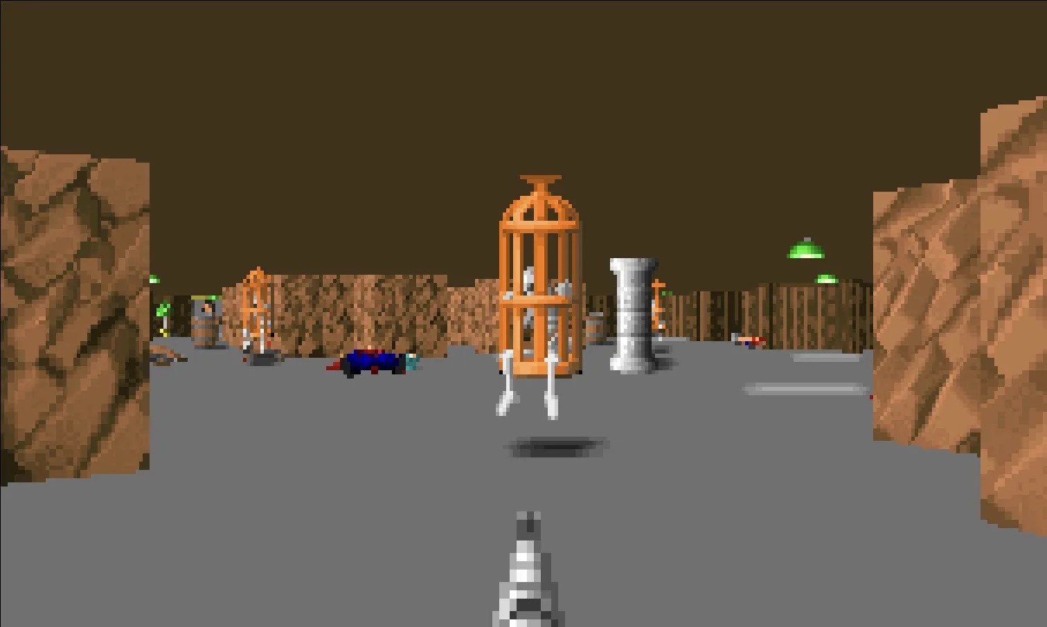
Wolfenstein 3D stands out as a prime example of a game that extensively utilized this technique. In the process, rays were traced to identify the closest objects. The distances from the player’s position were then used to scale these objects appropriately within the player’s view.
Point-in-polygon problem
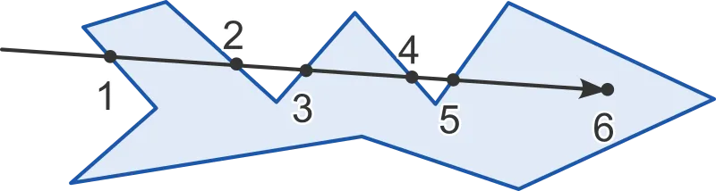
The PIP problem involves determining whether a given point is inside, outside, or on the boundary of a polygon. Using the ray casting algorithm, we can track the number of times the point intersects the edges of the polygon. If the count of intersections is even, the point is outside the polygon. Conversely, if the count is odd, the point is located either inside the polygon or on its boundary.
Object visibility and light casting
This section will cover fundamental concepts, including the calculation of intersection points, the process of casting rays, sorting intersection points to illuminate the visible area, and a brief discussion about circles.
Segment - ray intersection point
Let’s get into intersection points. We’ll break it down step by step, figuring out how to find them and make good use of them. First up, we’ll discuss a line’s parametric equation. Then, we’ll dive into the fun part – calculating the points. To wrap it up, we’ll chat about a smart way to figure out which one of these points is the closest.
Deriving line parametric equation
We can express vector by the following equation: , where is an equation parameter defining how much do we stretch, shrink, or if we flip the direction of vector in relation to vector .
Let’s get through with an example:

As you might have noticed, we can use as a scale factor: , where denotes the euclidean distance between two points. We’ll make good use of that fact when figuring out which intersection point is the closest.
Now we can easily see, that if we want the point to be contained on:
- line -
- ray -
- segment -
If you still do not know what happens here, I can recommend an awesome short lecture by Norm Prokup.
Calculating the intersection point
Let’s consider point as the intersection point between the segment defined by points and and the ray defined by points and . The expression for point can then be represented by a set of two equations:
- , where ,
- , where .
By solving for and , we obtain:
Next, we can calculate using one of the equations from the set.
Finding the closest intersection point
To find the closest intersection point for properly drawing the visible area, a straightforward approach involves calculating distances between the ray starting point and intersection points using the Pythagorean Theorem: . However, taking into account the line equation parameter , we can use it as a scale factor. To compare distances along the ray, we simply check for the smallest parameter value: .
Casting rays
Casting rays by offset angle
One approach is to cast rays in all directions with a specified offset angle. For example, we could cast a total of 30 rays, each offset by 12°. Let’s start by exploring how to generate all these rays.
Let be an anchor point of our rays, and let be a point on a line going through at an angle :
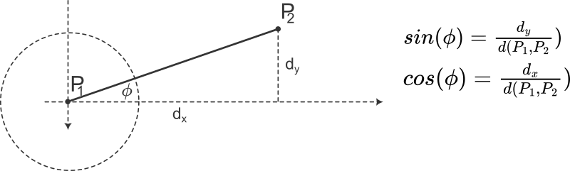
Let’s define and (inverted y-axis).
Using the image above, we can derive formulas for and :
- ,
- .
In our case, the distance has an arbitrary (greater than 0) value, as we are looking for any point on the line. Therefore, we can safely assume to simplify the calculations. Taking this into consideration, where is our angle offset.
Casting rays on vertices
Casting rays on vertices is probably your preferred approach. Rather than casting rays in all directions, we can simplify the process by casting them directly on the vertices of our polygons. This approach, depending on the number of vertices, allows us to conserve computing power by avoiding unnecessary ray casts. It will be the only method utilized in the upcoming sections.
Illuminating the visible area
Get ready for the exciting part! We’re about to light up the visible area by filling in a massive polygon.
Sorting intersection points
To arrange vertices correctly and construct a proper polygon, we need to first sort them by angle. For this, we’ll utilize the atan2(y, x) function.
Now, let’s check how it looks:
It seems to be glitchy, jumpy, and inaccurate. Let’s investigate the underlying reasons for these issues.
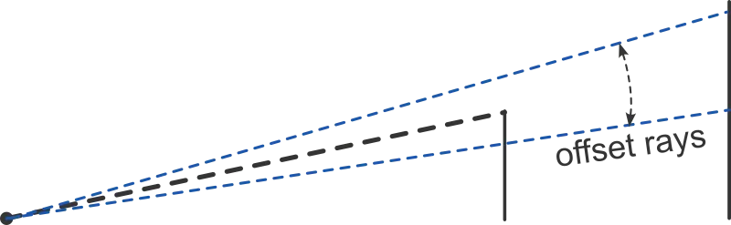
Casting slightly offset rays
Take note of what occurs when rays are cast directly onto vertices - they are expected to extend beyond that vertex, but we are currently only obtaining the closest intersection point. A common solution involves casting two additional rays offset by a small angle (in both directions) for every primary ray cast.
Consider a ray R starting at and going through . We aim to find a point such that the ray R would be rotated by an angle with A being the origin point. The coordinates of C would be as follows:
For further explanation you can check this article.
Introducing flashlight
To restrict the player’s visibility, we can establish a clipping region in the desired shape. In the demonstrations below, I utilized the CanvasRenderingContext2D.clip() method.
Optimization techniques
In this section, we will explore the utilization of spatial hashmaps and a modified Bresenham’s line algorithm. I won’t delve into implementation details, as they are readily available on the Internet. Nevertheless, I’ll provide you with some demos to experiment with and encourage you to come up with your own ideas on how to apply these techniques.
Spatial hashmaps
Currently, we are drawing all polygons and calculating all intersection points, but this is often inefficient. Typically, our play area will be much larger than the viewport. By implementing spatial hashmaps, we can easily identify which polygons are visible to the player and carry out appropriate calculations.
Essentially, the idea is to partition the play area into smaller cells of a predefined size. Each cell comprises a list containing our shapes, which are most likely line segments. If a single shape spans across multiple cells, it will be included in all of them.
Although the technique’s name suggests using hashmaps, in our case, employing a simple 2D array is more practical.
Below is a basic demo illustrating how this approach might function:
Bresenham-based supercover line algorithm
It’s about time we address the matter of finding the closest intersection points. By incorporating spatial hashmaps and a modified Bresenham’s line algorithm, we can navigate the grid efficiently, minimizing the number of checks needed. The algorithm should halt as soon as the first cell with an intersection point is discovered.
Read more about Bresenham’s line algorithm here, and its modified version here.
Everything has an end
I believe I’ve covered everything to assist you in getting started. I’ll do my best to expand on it in the future if I identify areas that need additional explanation.
If you enjoyed the content, be sure to follow me for more similar content in the future. Also, don’t hesitate to reach out if you find any topic poorly explained or if you have other suggestions.
See you!